
Excel Pivot Table
|
|
|
|
|
|
|
|
|
|
|
|
|
|
Excel Pivot Table
Additional Resources
Excel Pivot Table
Format an Excel Pivot Table | Microsoft Excel XP |
 |
 |
What's on this page... Formatting a PivotTable with AutoFormat Format cells in a PivotTable See also... Create a Pivot Table Change Layout of Pivot Table Calculating Fields Calculating Items |
Formatting A PivotTable With AutoFormat
When you create an Excel pivot table, you have an option of applying a default table AutoFormat.After the pivot table is created, you can specify a different AutoFormat.
Excel comes with a PivotTable AutoFormat feature that provides 22 pivot table AutoFormats.
To change or use an AutoFormat after the pivot table is created, follow these steps:
| 1. | Select any cell within the pivot table. |
| 2. | Select Format ► AutoFormat
from the menu bar. OR Choose PivotTable ► Format Report from the PivotTable toolbar.  PivotTable button
OR Click the Format Report button on the PivotTable toolbar. |
| This command opens up the AutoFormat dialog box with a list of PivotTable AutoFormats. | |
 |
|
| 3. | Choose any of the different AutoFormats from the preset list. |
| 4. | Click OK. |
The selected AutoFormat will add formatting to all the cells in the PivotTable.
|
|
Unsatisfied
with the AutoFormat that you have chosen? Simply go back to the AutoFormat dialog box and choose another! |
|
|
Use one of the AutoFormats labeled Report 1
up to
Report 10 when you want to display and/or print a report in indented format. Selecting an indented format changes the layout of your report. |
Formatting Cells In A PivotTable
When Excel creates a Pivot Table Report, it does not retain any special number formatting that you may have applied to your original data.For example, if you apply a currency format to your data and then use that data in the pivot table, the currency formatting is not retained in the pivot table.
To change the number format of cells in the Pivot Table, follow these steps:
| 1. | Select any cell in the pivot table's data area. |
| 2. | Right-click and choose Field Settings from the
shortcut menu. OR Click the Field Settings button on the PivotTable toolbar. |
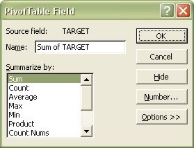
| Excel displays its' PivotTable Field dialog box. | |
 |
|
| 3. | Click the Number button. |
 |
|
| 4. | Select the Number Format that you need from the Categories list. |
| 5. | Click OK, and then click OK again to return to the PivotTable report. |
| See also... Creating a PivotTable | Change Layout of PivotTable |
| Calculating in a PivotTable |
| Back to Top |
| Return to Excel XP from Format an Excel Pivot Table |
Excel XP Topics
- Tips- Excel Screen Layout
- Navigational Techniques
- Working with Workbooks
- Templates
- Working with Worksheets
- Moving Around
- Move Worksheets
- Copy Worksheets
- Insert & Delete Cells
- Insert & Delete Rows
- Insert & Delete Columns
- Resize Row
- Resize Column
- Editing Data
- Content Color
- Cell Color
- Number Formats
- Fonts
- Alignment
- Text Direction
- Indent Contents
- Merge Cells
- Copy
- Move
- Undo & Redo
- Using Zoom
- Freeze & Unfreeze Titles
- Split Worksheet
- Spreadsheet Data
- AutoFill
- AutoComplete
- Comment
- Find
- Replace
- Spellcheck
- Formulas
- Functions
- Password
- Sorting
- AutoFilter
- Advanced Filter
- Macros
- Charts
- Charting
- Charting Elements
- Gantt Chart
- PivotTable
- PivotTable Calculations
- PivotTable Layout
- PivotTable Format
- PDF to Excel
- PDF-to-Excel Converter
- Excel to PDF Converter