
Excel Pivot Table
|
|
|
|
|
|
|
|
|
|
|
|
|
|
Additional Resources
Excel Pivot Table | Microsoft Excel XP |
 |
You haven't had any fun in Excel until you get to use pivot tables.
Why, you ask? Well, the name sounds as if you are doing something really complicated, so impressing your family and professional colleagues is very easy.
"Mr. Taylor, I'd like to have the McKinley report on your desk by tomorrow morning, but I have to create a pivot table in order to perform a dynamic summary of my data" (Note: If you're trying to impress your family, substitute Mom or any relevant title for Mr. Taylor.)
If only they knew the truth. Excel makes creating and using pivot tables as easy as choosing a few menu options and clicking buttons here and there on some simple dialog boxes. All you have to do is to provide the data.
 |
What's on this page... Pivot Table Creating a Pivot Table See also... Format a Pivot Table with AutoFormat Format a Pivot Table's Cells Change Layout of Pivot Table Calculating Fields Calculating Items |
Excel Pivot Table
An Excel Pivot Table is a dynamic summary of data contained in a database (contained on a worksheet or in an external file).An Excel pivot table lets you create frequency distributions and cross-tabulations made up of several different data dimensions.
In addition, you can display subtotals at any level of detail you desire.
Generally speaking, fields in a database table can be one of two types:
| ► | DATA - Contains a Value. |
| ► | CATEGORY - Describes the data. |
A database table can have any number of data fields and any number of category fields.
When you create an Excel pivot table, you usually want to summarize one or more of the data fields.
The values in the category fields appear in the Excel pivot table as rows, columns, or pages.
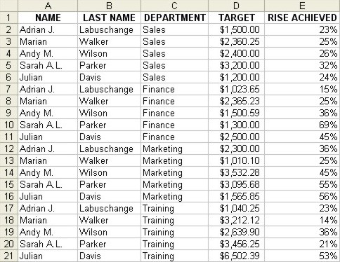
The image below shows an example of data necessary for creating an Excel pivot table.
 |
Creating A Pivot Table
To create an Excel pivot table from a worksheet database, follow these steps:
| 1. | Select all the data of the database from which you want to create a pivot table. |
| 2. | Choose Data ► PivotTable and PivotChart Report from the menu bar. |
| The PivotTable and PivotChart Wizard - Step 1 of 3 | |
 |
|
| 3. | Make
sure that the option labeled Microsoft Excel List or
Database and PivotTable are selected. If the data is in an external database, select the External Data Source option. The data is retrieved using MS Query (a separate application), and you'll be prompted for the data source in the second PivotTable Wizard dialog box. Click Next. |
 |
|
| 4. | In Step 2 of the Wizard, ensure that the Database Ranges is specified correctly and click Next. |
 |
|
| 5. | In
Step 3 of the Wizard, specify the location for the
pivot table. You can have the Excel Pivot Table on a separate New Worksheet. OR On the Existing Worksheet, click the starting cell on the current worksheet. |
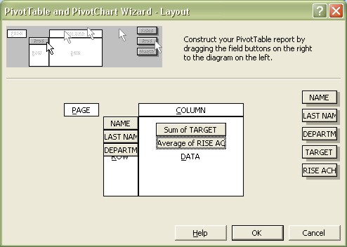
| 6. | Click the Layout button. |
 |
|
| 7. | Drag the field names from the
right side of the window to the appropriate drop zones. The ROW and COLUMN drop zones are usually used for field names that contains data. The DATA drop zones are used for field names with data that you can calculate with. |
 |
|
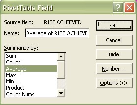
| You'll notice that when
you drag field names to the DATA area, it shows "Sum of...". You can change the function by double clicking on the field name. Select the function from the list and click OK. |
|
| 8. | Once you're happy with the layout of the pivot table, click OK. |
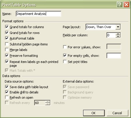
| 9. | Click the Options button. |
 |
|
| 10. | Excel includes several options for pivot tables: |
| ►
AUTOFORMAT
TABLE Check this box if you want Excel to apply a default AutoFormat to the pivot table. Excel uses the AutoFormat even if your rearrange the table layout. ► SUBTOTAL HIDDEN PAGE ITEMS Check this box if you want Excel to include hidden items in the Page Fields in the subtotals. ► MERGE LABELS Check this box if you want Excel to merge the cells for outer row and column labels. Doing so may make the table more readable. ► PRESERVE FORMATTING Check this box if you would like Excel to keep any formatting that you applied when the pivot table is updated. ► REPEAT ITEM LABELS ON EACH PRINTED PAGE Check this box if you want Excel to repeat item labels on each page for all rows to the left of the field for which a page break separates a group of items. ► PAGE LAYOUT Specify the order in which you want the page fields to appear. ► FIELDS PER COLUMN Specify the number of page fields to show before staring another row of page fields. ► FOR ERROR VALUES, SHOW You can specify a value to show for pivot table cells that display an error. ► FOR EMPTY CELLS, SHOW You can specify a value to show for pivot table cells that are empty. ► SET PRINT TITLES Check this box if you want Excel to repeat row labels, column labels, and item labels on each page of a PivotTable report. This option is applicable only for Excel Pivot Table reports in indented format. Also, Page Setup options used to repeat rows and columns should be cleared. ► SAVE DATA WITH TABLE LAYOUT If this option is checked, Excel stores an additional copy of the data (called a pivot table cache) to allow it to recalculate the table more quickly when you change the layout. If memory is an issue, keep this option unchecked (updating will be a bit slower). ► ENABLE DRILL DOWN If checked, you can double-click a cell in the pivot table to view details. ► REFRESH ON OPEN If checked, the pivot table is refreshed whenever you open the workbook. ► REFRESH EVERY XXXX MINUTES To periodically refresh a report based on external data, check this box and then enter the interval you want in the minutes box. This check box is unavailable for reports based on Excel source data. Minutes can range from 1 to 32676 inclusive. ► SAVE PASSWORD If you use an external database that requires a password, this option enables you to store the password as part of the query so you wont have to enter it. ► BACKGROUND QUERY If checked, Excel runs the external database query in the background while you continue your work. ► OPTIMIZE MEMORY This option reduces the amount of memory used when you refresh an external database query. |
|
| 11. | Once your options are set click OK. |
| 12. | Click Finish. |
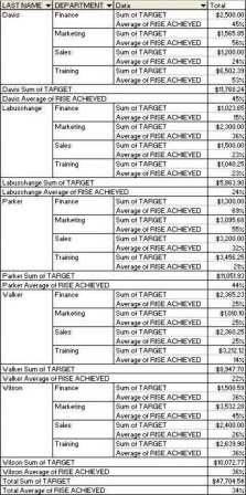
A resulting Excel pivot table of the above data table will look like this:
 |
| See also... Format a PivotTable |
| Change Layout of a PivotTable | Calculating in a PivotTable |
| Back to Top |
| Return to Excel XP from Excel Pivot Table |
Excel XP Topics
- Tips- Excel Screen Layout
- Navigational Techniques
- Working with Workbooks
- Templates
- Working with Worksheets
- Moving Around
- Move Worksheets
- Copy Worksheets
- Insert & Delete Cells
- Insert & Delete Rows
- Insert & Delete Columns
- Resize Row
- Resize Column
- Editing Data
- Content Color
- Cell Color
- Number Formats
- Fonts
- Alignment
- Text Direction
- Indent Contents
- Merge Cells
- Copy
- Move
- Undo & Redo
- Using Zoom
- Freeze & Unfreeze Titles
- Split Worksheet
- Spreadsheet Data
- AutoFill
- AutoComplete
- Comment
- Find
- Replace
- Spellcheck
- Formulas
- Functions
- Password
- Sorting
- AutoFilter
- Advanced Filter
- Macros
- Charts
- Charting
- Charting Elements
- Gantt Chart
- PivotTable
- PivotTable Calculations
- PivotTable Layout
- PivotTable Format
- PDF to Excel
- PDF-to-Excel Converter
- Excel to PDF Converter