Excel Charting Elements
|
|
|
|
|
|
|
|
|
|
|
|
|
|
Excel Charting Elements
Additional Resources
Excel Charting Elements
Excel Charting Elements | Microsoft Excel XP | Page 3 |
 |
 |
What's on this page... Dealing with Chart Elements Modify a Chart Element Move a Chart Element Deleting a Chart Element Chart Basics Adding a new Data Series to a chart Changing the Chart's Data Series Working with chart Legends Changing a chart's Scale Changing a chart's Gridlines Rotating and Elevating a 3D Chart See also... Excel Charts Excel Charting with the Chart Wizard |
Changing The Charts Data Series
The data series are one of the most important parts of all the Excel charting elements. Often, you create a chart that uses a particular range of data, and then you extend the data range by adding new data points in the worksheet.When you add new data to a range, the new data won't be included in the data series.
Or you may delete some of the data points in a range that is plotted.
If you delete data from a range, the chart displays the deleted data as zero values.
To update the chart to reflect the new data range, follow these steps:
| 1. | Activate the chart. |
| 2. | Choose Chart ► Source Data from the menu bar. |
 |
|
| 3. | Select the Data Range tab of the Source Data dialog box and specify the data range for the entire chart. |
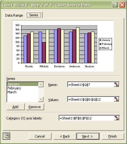
| 4. | In the Source Data dialog box select the tab labeled Series. |
| 5. | Select the data series that you want to modify from the list labeled Series. |
| 6. | Use the range selection buttons to change the data series. You may also need to modify the range used for the Category values. |
|
|
|
| 7. | Click OK, and the chart are updated with the new data range. |
When you activate a chart, the range used by the chart, are outlined in the worksheet. To extend or reduce the range, simply drag the handle, located at the corner of the outline, in the worksheet.
 |
 |
A better way to handle data ranges that change is to use named ranges. Simply create names for the data ranges that you use in the chart. Activate the chart, select the data series, and edit the SERIES formula by clicking the formula bar. Replace each range reference with the corresponding range name. If and when, you change the definition for a name, the chart is updated. |
Excel XP Topics
- Tips- Excel Screen Layout
- Navigational Techniques
- Working with Workbooks
- Templates
- Working with Worksheets
- Moving Around
- Move Worksheets
- Copy Worksheets
- Insert & Delete Cells
- Insert & Delete Rows
- Insert & Delete Columns
- Resize Row
- Resize Column
- Editing Data
- Content Color
- Cell Color
- Number Formats
- Fonts
- Alignment
- Text Direction
- Indent Contents
- Merge Cells
- Copy
- Move
- Undo & Redo
- Using Zoom
- Freeze & Unfreeze Titles
- Split Worksheet
- Spreadsheet Data
- AutoFill
- AutoComplete
- Comment
- Find
- Replace
- Spellcheck
- Formulas
- Functions
- Password
- Sorting
- AutoFilter
- Advanced Filter
- Macros
- Charts
- Charting
- Charting Elements
- Gantt Chart
- PivotTable
- PivotTable Calculations
- PivotTable Layout
- PivotTable Format
- PDF to Excel
- PDF-to-Excel Converter
- Excel to PDF Converter